Knowledge note
Microscaling (MX) Formats: Block Floating Point for AI Hardware
A source-backed history and hardware reading of MX block floating point, from FPGA-era MSFP through OCP's 32-element MXFP4, MXFP6, MXFP8, and MXINT8 formats.
Microscaling (MX) Formats: Block Floating Point for AI Hardware
Paper: OCP Microscaling Formats (MX) Specification v1.0 Authors: OCP MX consortium contributors from AMD, Arm, Intel, Meta, Microsoft, NVIDIA, and Qualcomm Version: 1.0 (2023-09-07)
Related pages: Microscaling · Quantization · HiFloat4 (HiF4) · NVFP4: Blackwell 4-Bit Floating Point · Spatial GEMM
TL;DR
What: The OCP MX specification builds a vector data type from one shared scale, same-type private elements, and a fixed scaling block size. How: Its concrete formats use 32 elements and an 8-bit E8M0 scale, while the element payload is FP4, FP6, FP8, or INT8 and the physical layout remains implementation-defined. The number: One MXFP6 block is $32 \times 6 + 8 = 200$ bits; the specification also requires a supported implementation to provide the listed conversion and dot-product semantics.
The Big Picture
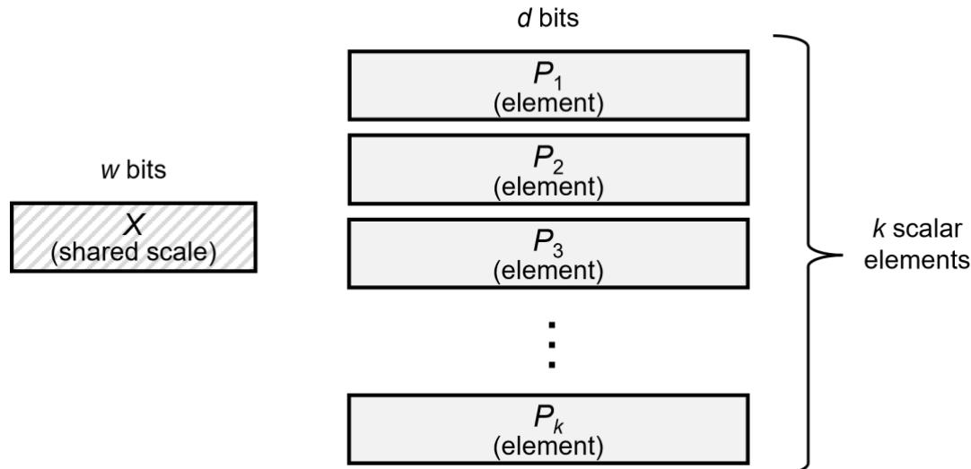
Source: Section 5.1 of the OCP Microscaling Formats specification. 1. One scale X is shared by 2. k same-type scalar elements P_i; 3. the encoded block occupies (w + k*d) bits, while the specification leaves its physical memory layout open.
The important boundary is visible in the figure: MX is a block floating point vector data type assembled from a scale encoding, a private element encoding, and a block size. It is not simply “FP4” or “FP8” applied independently to every value.
Why This Exists
Consider one vector dot product implemented with ordinary floating-point elements. Each product has its own exponent, and the reduction tree must repeatedly align products before adding them. Those alignment shifters and normalization steps can dominate a narrow-precision FPGA implementation even when the multipliers themselves are small. A shared block exponent lets the datapath align many products once, while narrow element multipliers map efficiently to LUTs and DSP blocks.
The tradeoff is equally concrete: if a block contains one large value and many small values, the shared scale must cover the block range. MX exists to choose a block size and private element format that make this loss acceptable for tensor workloads while making the data movement and dot-product hardware much cheaper.
The Landscape
flowchart LR
    WILK["Wilkinson 1963<br/>block-floating vectors"] --> BFP["Block floating point<br/>shared scale + narrow elements"]
    BFP --> MSFP["MSFP / Brainwave<br/>FPGA BFP and shared exponents"]
    MSFP --> OCP["OCP MX v1.0<br/>32 elements + E8M0 scale"]
    BFP --> BDR["BDR / shared microexponents<br/>ISCA 2023 MX4, MX6, MX9"]
    BDR -. "distinct from OCP MX formats" .-> OCP
    OCP --> ACCEL["Matrix-multiply hardware<br/>FPGA, ASIC, GPU, NPU"]
    OCP -. "related microscaling successor" .-> NVFP4["NVFP4<br/>16 elements + E4M3 + FP32 global"]
Synthesized landscape from the captured article and its cited papers. The solid path follows the article’s block-floating-point lineage; the dashed edge distinguishes the ISCA 2023 shared-microexponent designs from the later OCP MX Alliance formats and relates OCP MX to the NVFP4 page.
The Core Idea
Microscaling amortizes exponent metadata across a small block. Instead of paying for a full exponent with every scalar, the format stores one shared scale and spends the saved bits on more element values or cheaper hardware. The same choice also changes the dot product: common scaling removes much of the per-element alignment work, but the standard must still be paired with an implementation policy for layout, multiplication, accumulation, and operations outside the dot product.
Symbol Map
The specification uses E x M y to mean one sign bit, x exponent bits, and y fraction bits; the notation therefore describes a total floating-point element width of 1 + x + y bits. The M count is the fraction field rather than the implicit leading bit. E8M0 is the unsigned scale encoding and therefore has no sign bit.
| Symbol | Human name | Shape / scope | Plain meaning |
|---|---|---|---|
| $X$ | shared scale | one per block | Common scale or exponent encoding applied to every element in the block. |
| $P_i$ | private element | one of $k$ elements | Same-type narrow element carrying the block’s per-value payload. |
| $k$ | block size | elements per block | Number of private elements sharing $X$; OCP MX uses $k=32$. |
| $w$ | scale width | bits per block | Number of bits used to encode $X$; OCP MX uses 8 bits. |
| $d$ | element width | bits per element | Number of bits used for each $P_i$; the format family selects 4, 6, or 8. |
| $C$ | dot-product result | scalar | Result of an MX vector dot product or the general dot product. |
E4M3 |
FP8 element encoding | 8-bit scalar | One sign bit, four exponent bits, and three fraction bits. |
E8M0 |
shared-scale encoding | 8-bit scale | Unsigned biased Float32 exponent with supported exponent range -127 to 127. |
MXFP4, MXFP6, MXFP8 |
MX floating-point formats | 32-element vector block | OCP MX formats whose private elements are FP4, FP6, or FP8. |
MXINT8 |
MX integer format | 32-element vector block | OCP MX format whose private elements are signed 8-bit integers. |
For finite scale and element encodings, reconstruction has the form
\[v_i = X \cdot \operatorname{decode}(P_i)\]If X is NaN, every value in the block is NaN and the element encodings are ignored. Values outside the Float32 range, the exact product interpretation, accumulation precision, and operation order are implementation choices where the specification is intentionally incomplete.
Deep Dive
Shared-scale block encoding
What it does: Builds a vector data type from one scale encoding and $k$ same-width private elements.
Why it matters: The shared scale is the mechanism that trades per-element exponent storage and alignment logic for a block-level approximation.
How it works:
- Choose a scale encoding of width $w$, a private element encoding of width $d$, and a block size $k$.
- Encode one shared scale as $X$ and each value as a private element $P_i$ relative to $X$.
- Store or stream the scale and the $k$ elements using any implementation-defined physical layout.
- Reconstruct each value from the scale and its private element, subject to the specification’s NaN and Float32-range rules.
The encoded block costs $w + k d$ bits. OCP MX fixes $w=8$ and $k=32$, but the scale and element encodings remain separate choices.
The intuition: Pay for the ruler once, then measure a whole tray of values with it.
A concrete example: For MXFP6, one 8-bit scale accompanies 32 six-bit elements, so the block consumes 200 bits instead of 32 independent floating-point records with separate exponents.
Remember: MX is a block representation, not a single scalar precision.
Why common exponents help FPGA dot products
What it does: Removes much of the exponent-alignment work from a narrow-precision multiply-accumulate pipeline.
Why it matters: In the source’s FPGA analysis, multiplication is relatively cheap; the adder tree’s alignment shifters, normalization, and extra pipeline stages are the harder resource problem.
How it works:
- Decode the shared block scale once rather than aligning every product from unrelated exponents.
- Multiply narrow element payloads with LUT- or DSP-friendly circuits.
- Convert or align products into the chosen accumulation domain.
- Reduce the products with a fixed-point or other implementation-selected accumulator.
The captured article connects this design to Microsoft’s Brainwave architecture, which used shared-exponent MSFP/BFP variants and reported up to 96,000 MACs on a Stratix 10-280 FPGA. It also cites a 90 TOPS ms-fp8 result at 720 GFLOPS/W; those are cited historical results, not measurements performed by this repository.
The intuition: Shared exponents move expensive alignment out of the innermost MAC loop.
A concrete example: A four-term reduction whose products have unrelated exponents needs a pre-addition shifter at every merge. If the terms share a block scale, the hardware can keep the reduction in a narrower, more regular domain.
Remember: The hardware win comes as much from cheaper addition and alignment as from smaller multiplication.
The OCP MX format family
What it does: Standardizes a small set of 32-element block formats for matrix multiplies and convolutions.
Why it matters: The family gives hardware and software a common target across vendors while preserving multiple accuracy and cost points.
How it works: Every row below uses the same 8-bit E8M0 scale and 32-element block. The private element type changes the payload width and numerical behavior.
| Format | Private element encoding | Element bits $d$ | Block size $k$ | Scale | Encoded block bits |
|---|---|---|---|---|---|
MXFP4 |
E2M1 |
4 | 32 | E8M0 |
136 |
MXFP6 |
E3M2 or E2M3 |
6 | 32 | E8M0 |
200 |
MXFP8 |
E4M3 or E5M2 |
8 | 32 | E8M0 |
264 |
MXINT8 |
signed integer | 8 | 32 | E8M0 |
264 |
An implementation does not need to support every concrete format. For each format it does support, it must support the parameters listed in the specification; the E4M3 and E5M2 variants of MXFP8, and the E3M2 and E2M3 variants of MXFP6, count as separate formats. The accompanying whitepaper reports that MXFP6 can approach FP32 inference after quantization-aware fine-tuning and that MXFP4 weights with MXFP6 activations and gradients can train with a minor loss penalty, but those claims depend on the cited workloads and recipe.
The intuition: The block size stays fixed while the element type lets a deployment choose where to spend its bit budget.
A concrete example: MXFP4 saves 64 bits per block versus MXFP6, while MXFP6 retains two more bits per element for activations or gradients that are more sensitive to quantization error.
Remember: MXFP4, MXFP6, and MXFP8 differ in private element encoding; the shared scale and block size stay the same.
Conversion and exceptional values
What it does: Defines the minimum conversion behavior needed to create MX blocks from scalar vectors.
Why it matters: A shared-scale format is only useful when different implementations agree on how values are scaled, rounded, clamped, and represented at the edges of the range.
How it works: For a length-$k$ scalar vector $V$, the specified baseline conversion is:
- Set $X$ to the largest power of two less than or equal to the maximum absolute input, divided by the largest power of two representable by the element type.
- Quantize each $V_i / X$ to the selected element type.
- Clamp normal values beyond the element type’s maximum normal magnitude, preserving sign.
The implementation must support roundTiesToEven; other rounding modes may also be available. The element-specific rules are:
| Element type | Normative details |
|---|---|
| FP8 | Follows the OCP FP8 encoding and must support both saturating and overflow conversion modes. |
| FP6 / FP4 | Supports subnormals, has no Inf or NaN encodings, rounds with roundTiesToEven, clamps overflow, and converts values below the minimum subnormal magnitude to zero. |
| INT8 | Uses two’s-complement encoding with an implicit $2^{-6}$ scale; it rounds with roundTiesToEven, clamps overflow, and may leave the most-negative code unused to keep the range symmetric. |
| E8M0 | Uses bias 127 over exponents -127 to 127; all ones is the single NaN encoding, with no zero or Inf encoding. |
Conversion from NaN is implementation-defined. If the block scale itself is NaN, every value in the block is NaN and the private element encodings are ignored.
The intuition: The scale chooses the ruler, while the element format determines how finely that ruler can mark the block.
A concrete example: MXFP4 can represent only a few values after scaling, so its 32-element block saves 64 bits versus MXFP6 but gives up two payload bits per element.
Remember: The format standardizes edge behavior and rounding requirements, but not the algorithmic choices applications make before conversion.
Dot products factor out the scales
What it does: Defines the minimum dot-product semantics for two MX vectors.
Why it matters: The shared scales can be applied outside the reduction, leaving the inner sum to operate on narrow private elements.
How it works: For two length-$k$ MX vectors $A$ and $B$, the result is minimally defined as
\[C = \operatorname{Dot}(A, B) = X^{(A)} X^{(B)} \sum_{i=1}^{k} \left(P_i^{(A)} \times P_i^{(B)}\right)\]The two vectors may use different scale and element data types. A general dot product pads vectors to a multiple of $k$, splits them into MX sub-vectors, and sums their block dot products; that general result should be a scalar Float32. The internal precision and operation order of both the block reduction and intermediate general-dot sums are implementation-defined.
The intuition: Shared scales are multiplied once per block, so the reduction can focus on the narrow payloads.
A concrete example: MXFP4 weights and MXFP6 activations can feed an asymmetric dot product, but the surrounding implementation still has to choose the accumulator and reduction order.
Remember: MX specifies the mathematical shape of the dot product, not a bit-exact kernel implementation.
The specification boundary
What it does: Defines the common ingredients of an MX-compliant block without fixing every kernel-level decision.
Why it matters: A format can be widely adopted while still producing different numerical results across libraries, accelerators, or FPGA cores if their hidden implementation choices differ.
How it works: The specification deliberately leaves several implementation choices open:
- the physical in-memory layout of the scale and elements;
- the internal and final precision of an MX dot product, plus the order of accumulation;
- the complete set of required MX operations beyond conversion and dot product.
The captured article treats this freedom as a portability and reproducibility risk. That is a useful critique, not a claim that every implementation is incorrect: vendors may need room to map one logical format onto very different CPUs, GPUs, NPUs, and FPGA fabrics. The practical boundary is that two compliant implementations can agree on the block representation while still producing different numerical results or requiring different packing and conversion code.
The intuition: OCP standardizes the shape of the envelope, but not the entire machine inside it.
A concrete example: Two compliant dot-product units can use different accumulator widths or reduction orders and therefore produce slightly different results for the same MX blocks.
Remember: MX compliance does not by itself define a canonical byte layout or bit-exact dot product.
From FPGA BFP to co-designed AI silicon
What it does: Shows how the shared-scale idea moved from FPGA implementations into a broader hardware and model-design story.
Why it matters: MX is easier to understand as hardware-software co-design than as an isolated quantization format.
How it works: The article’s historical path is:
- Project Catapult established large-scale datacenter FPGA deployment experience.
- Project Brainwave used FPGA-friendly MSFP/BFP representations, shared exponents, vector parallelism, and specialized reduction networks.
- Later MSFP work evaluated accuracy and area/energy tradeoffs, including MSFP12 and MSFP16.
- Commercial FPGA products added hardened or configurable block-floating-point dot-product resources.
- The ISCA 2023 shared-microexponent work explored a related but distinct BDR design space, including MX4, MX6, and MX9.
- Microsoft Maia 100 is cited as a later custom accelerator supporting sub-8-bit MX data types.
The article presents this as a perspective on why FPGA constraints can reveal useful ASIC and accelerator design tradeoffs. The causal interpretation is the author’s synthesis; the individual projects and cited papers are the direct evidence.
The intuition: When the fabric makes ordinary floating point expensive, the data representation becomes part of the architecture.
A concrete example: A system may keep weights in MXFP4 and activations in MXFP6, so the accelerator needs an asymmetric input dot product rather than one universal element type.
Remember: MX is a joint choice about models, memory, arithmetic, and silicon.
Compute-flow boundary: MX inside GEMM, wider types around it
What it does: Places MX where its shared-scale arithmetic is most useful while keeping wider formats for general vector operations.
Why it matters: Treating an MX deployment as “the whole model is 4-bit” hides the conversions and higher-precision operations that make the system usable.
How it works:
- Quantize weights or activations from BF16 or FP32 into MX blocks along the relevant reduction dimension.
- Feed the blocks to many MX vector dot products inside a GEMM or convolution.
- Accumulate and return a wider result such as BF16.
- Keep elementwise operations, softmax, and other numerically sensitive paths in BF16 or FP32 where required by the workload.
The specification defines conversion and dot products, but does not require MX for every operation; weights and activations can also use different MX representations.
The intuition: MX is specialized fuel for the matrix engine, not necessarily the language spoken by every layer around it.
A concrete example: MXFP4 weights reduce storage, MXFP6 activations preserve more dynamic information, and BF16 remains the surrounding tensor format after the dot products.
Remember: The conversion and accumulation path is part of the format story.
Putting It Together
Trace one matrix-multiply tile through an MX-enabled accelerator:
- Choose the contract: Select the private element type, the shared E8M0 scale, and the 32-element block size.
- Quantize: Convert a BF16 or FP32 vector into one scale plus 32 private elements for each block.
- Move data: Store the scale and payload in the accelerator’s chosen layout; the OCP specification does not prescribe the byte order.
- Compute: Decode the scale, multiply narrow elements, and accumulate each block’s contribution with the implementation’s chosen internal precision.
- Reduce: Sum block-level dot products into the wider result expected by the matrix-multiply pipeline.
- Continue the model: Run surrounding normalization, softmax, or elementwise work in BF16 or FP32 as required, then quantize the next matrix operand.
- Validate the deployment: Compare accuracy and reproducibility across the exact kernels, accumulation order, and mixed-format choices used in production.
What This Buys You
The headline claim
The OCP specification makes MX a portable logical contract for sub-8-bit tensor math: it standardizes the block ingredients, concrete encodings, conversion minimums, and dot-product shape while leaving hardware mapping choices open.
How we know: cited format and hardware evidence
| Evidence | What it supports | How to read it |
|---|---|---|
| OCP Table 1 | Four concrete families: MXFP4, MXFP6, MXFP8, and MXINT8 | Direct specification coverage; an implementation may support a subset. |
| OCP Sections 5.1 and 6.1 | Shared-scale reconstruction and scale-factored dot products | Direct semantics, but not a canonical memory layout or accumulator. |
| Brainwave reports up to 96,000 MACs and 90 TOPS ms-fp8 | Shared-exponent FPGA datapath efficiency | Historical architecture results cited by the article, not a current benchmark. |
| MSFP12/MSFP16 area and energy comparisons | Hardware cost can fall at similar accuracy | Results depend on the cited synthesis and model settings. |
| MXFP6 and mixed MXFP4/MXFP6 training claims | Quantization-aware training can recover quality | The whitepaper’s workloads and recipe define the result. |
The mechanism behind the numbers
The gains come from several effects reinforcing one another: the scale is stored once per block, narrow products map to compact multipliers, shared exponents reduce alignment shifters in the reduction tree, and block-level quantization makes memory traffic smaller. Accuracy survives when the block size, element format, calibration, and model workload keep the shared-scale error within tolerance.
How to read these numbers
The specification itself is not a benchmark paper. The historical results are source-reported claims from papers, product material, and an expert essay captured in 2026; they establish design rationale, not a current kernel guarantee. In particular, the open accumulation and layout choices mean that two implementations can have different performance and numerical behavior while both claiming MX compatibility.
Where It Breaks
| Failure mode | When it happens | Impact |
|---|---|---|
| Shared-scale outlier | One element dominates the range of a 32-element block | Smaller values lose effective precision. |
| Format used outside its sweet spot | MX is applied to elementwise, softmax, or other non-GEMM operations without a suitable wider path | Accuracy or throughput can degrade; MX may not be the right representation. |
| Layout ambiguity | Software assumes a universal byte order for MX blocks | Kernels and libraries need format-specific packing and conversion logic. |
| Accumulation ambiguity | Implementations choose different internal precision or reduction order | Results can diverge across devices and libraries. |
| Mixed-format mismatch | Weights, activations, and gradients use incompatible block or element choices | The accelerator needs extra conversion or asymmetric dot-product support. |
| Historical evidence overgeneralized | Brainwave, MSFP, or whitepaper results are treated as universal guarantees | Modern models and hardware may not reproduce the cited accuracy, cost, or throughput. |
One Thing to Remember
MX is a block-level contract that turns floating-point tensor math into shared-scale narrow arithmetic: one scale amortizes metadata and alignment work across 32 elements, but the deployment still has to define layout, accumulation, conversion, and the wider operations around the matrix engine.
Go Deeper
- Read: FPGA.org: Microscaling (MX) Formats
- Read the specification: OCP Microscaling Formats (MX) Specification v1.0
- Read the evaluation: Microscaling Data Formats for Deep Learning
- Read the related design space: With Shared Microexponents, A Little Shifting Goes a Long Way
- Understand the newer format comparison: NVFP4 via NVFP4: Blackwell 4-Bit Floating Point
- Compare another shared-scale design: HiFloat4 (HiF4) uses 64 S1P2 values, an E6M2 base scale, and two levels of shared micro-exponents rather than OCP MX’s 32-value E8M0 block.
- Understand the hardware context: Spatial GEMM
- Reproduce: No local reproduction; this page records the captured article and its cited results.