mHC: Manifold-Constrained Hyper-Connections

Paper: mHC: Manifold-Constrained Hyper-Connections Authors: Zhenda Xie, Yixuan Wei, Huanqi Cao, Chenggang Zhao, Chengqi Deng, et al. (DeepSeek-AI) arXiv: 2512.24880

Related pages: DeepSeek-V4 · Hyper-Connections (term)

TL;DR

What: mHC keeps the performance gains of Hyper-Connections (HC) while restoring the identity-mapping property that unconstrained HC destroys, by constraining the residual mixing matrix to be doubly stochastic. How: The Sinkhorn-Knopp algorithm entropically projects each residual mapping onto the Birkhoff polytope of doubly stochastic matrices; because such matrices are non-expansive and closed under multiplication, composite signal gain stays bounded — and fused kernels, selective recomputation, and DualPipe overlap keep the added cost at 6.7%. The number: On a 27B MoE, mHC reaches a final loss 0.021 lower than the residual baseline and cuts HC’s composite signal gain from ~3000 down to ≤1.6.

The Big Picture

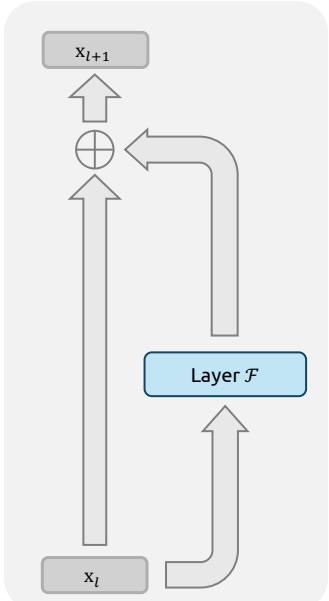
Source: Figure 1(a) of the paper. ① One $C$-wide stream carries the state. ② The layer function $\mathcal{F}$ writes its output back onto the same stream as an addition. ③ The identity path $\mathbf{x}_l \to \mathbf{x}_{l+1}$ is unimpeded — the property that keeps deep nets trainable.

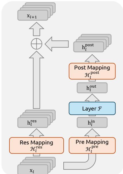
Source: Figure 1(b) of the paper. ① The stream is widened to $n \times C$. ② $\mathcal{H}^{\text{res}}$ mixes streams with a learned $n \times n$ matrix. ③ $\mathcal{H}^{\text{pre}}$ aggregates streams into the layer input; $\mathcal{H}^{\text{post}}$ writes the output back. Nothing constrains these mappings, so repeated application can amplify or shrink signal.

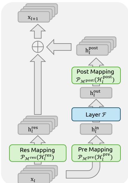
Source: Figure 1(c) of the paper. ① Identical $n$-stream topology to HC. ② The difference: $\mathcal{H}^{\text{res}}$ is projected onto the doubly stochastic manifold (Birkhoff polytope), so mixing is always a convex combination of streams. ③ This restores bounded signal propagation while keeping cross-stream information exchange.

The message of the figure is that the topology is unchanged from HC to mHC — only the constraint on the residual mapping differs, and that one change is what makes deep stacks stable.

Why This Exists

Imagine you are DeepSeek training a 27B-parameter MoE (DeepSeek-V3-style architecture). You adopt Hyper-Connections because the ablation in Table 1 of the paper shows the residual mixing mapping alone lowers loss by 0.022. Training starts fine — then, around step 12,000, the loss suddenly surges and the gradient norm spikes out of control. You check the residual stream and find that the composite mapping across 30 layers (60 sub-layers if you unroll attention and FFN separately) has a worst-case gain of ~3000×: some path is amplifying signal by three orders of magnitude. The identity-mapping property — the reason residuals are trainable at all — has silently vanished.

That is the pain mHC fixes: HC’s unconstrained residual matrices give better loss but break stability at scale. mHC is the fix that keeps the gain without the explosion.

The Landscape

flowchart TD
    RESNET[ResNet<br/>identity-mapping residual]
    DENSE[DenseNet] --> MACRO[Macro-design:<br/>dense / multi-path connectivity]
    FRACTAL[FractalNet] --> MACRO
    DLA[Deep Layer Aggregation] --> MACRO
    RESIDUAL[ResiDual] --> MACRO
    MACRO --> WIDEN[Widened residual stream]
    HIGHWAY[Highway Transformer] --> WIDEN
    DENSEFORMER[DenseFormer] --> WIDEN
    LAUREL[LAurel] --> WIDEN
    RMT[Residual Matrix Transformer] --> WIDEN
    MUDD[MUDDFormer] --> WIDEN
    HC[Hyper-Connections HC<br/>Zhu et al. 2024] --> WIDEN
    RESNET --> HC
    WIDEN --> PROBLEM[Unconstrained mixing<br/>breaks identity mapping]
    HC --> PROBLEM
    PROBLEM --> MHC[Manifold-Constrained HC<br/>mHC — this paper<br/>Sinkhorn-Knopp to Birkhoff polytope]
    MHC --> DSV4[DeepSeek-V4<br/>mHC deployed at 1.6T / 284B scale]

Editable source: mhc-landscape.mmd. The residual-connection lineage (ResNet → macro-design → widened streams) is the parent branch; HC is the direct parent; sibling widened-stream designs (Highway Transformer, DenseFormer, LAurel, RMT, MUDDFormer) share the instability problem; mHC is the constrained descendant that restores identity mapping and is deployed at scale in DeepSeek-V4.

The Core Idea

Hyper-Connections improve training by giving the residual stream more lanes and letting the network learn how to merge them — but an unconstrained mixing matrix, applied over dozens of layers, is a random signal amplifier. mHC keeps the lanes but locks the mixing to the set of doubly stochastic matrices: every stream’s signal is always a weighted average of the others. Averages can’t blow up, and a product of averages is still an average, so the identity-mapping property — the thing that made ResNet trainable — is restored at any depth. The entire paper is: widen the stream (HC’s idea), then constrain the mixer (mHC’s idea), then engineer away the extra memory and I/O cost so it’s nearly free.

Symbol Map

C (or $d$) = width of one residual stream / layer input; n = expansion rate (number of streams, 4 in the experiments); superscripts res / pre / post distinguish the three learnable mappings (residual mixer, read-out, write-back).

Symbol	Human name	Shape / scope	Plain meaning
$\mathbf{x}_l$	residual stream state	$n \times C$, per layer	The widened hidden state carried between layers.
$\mathcal{H}_l^{\text{res}}$	residual mixing matrix	$n \times n$, per layer	Mixes the $n$ streams; the matrix mHC constrains.
$\mathcal{H}_l^{\text{pre}}$	read-out mapping	$1 \times n$, per layer	Aggregates streams into the layer input $\mathbb{R}^{1 \times C}$.
$\mathcal{H}_l^{\text{post}}$	write-back mapping	$1 \times n$, per layer	Spreads the layer output back onto the $n$ streams.
$\mathcal{F}(\cdot, \mathcal{W}_l)$	layer function	$\mathbb{R}^{1\times C}\to\mathbb{R}^{1\times C}$	Attention or FFN block; unchanged by HC/mHC.
Birkhoff polytope	doubly stochastic manifold	subset of $\mathbb{R}^{n\times n}$	Non-negative matrices with rows and columns summing to 1.
Sinkhorn-Knopp(·)	projection operator	$\mathbb{R}^{n\times n}\to$ polytope	Iteratively rescales rows/columns until doubly stochastic.
Amax Gain Magnitude	instability metric	scalar per layer	Max abs row sum (forward signal) or column sum (backward gradient) of the composite mapping.

Cached vs. computed: the mapping coefficients ($\mathcal{H}^{\text{pre}}, \mathcal{H}^{\text{post}}, \mathcal{H}^{\text{res}}$) are cheap, input-dependent, and recomputed in the backward pass; the layer-function activations are the expensive part and are stored per layer.

Deep Dive

Hyper-Connections: the widened residual stream

What it does: HC replaces the single residual stream with $n$ parallel streams and three learnable mappings:

\[\mathbf{x}_{l+1} = \mathcal{H}_l^{\text{res}} \mathbf{x}_l + \mathcal{H}_l^{\text{post}^\top} \mathcal{F}(\mathcal{H}_l^{\text{pre}} \mathbf{x}_l, \mathcal{W}_l).\]

Why it matters: the residual stream’s information capacity is no longer tied to the layer width $C$ that drives FLOPs — you can scale the stream independently of compute.

How it works: each mapping is a dynamic (input-dependent) part plus a static bias, e.g. $\mathcal{H}_l^{\text{res}} = \alpha_l^{\text{res}} \cdot \tanh(\theta_l^{\text{res}} \tilde{\mathbf{x}}_l^\top) + \mathbf{b}_l^{\text{res}}$ with small-initialized gating $\alpha$. Since $n \ll C$, computing these costs negligible FLOPs.

The intuition: more lanes, learnable merges — the network decides how much of each stream feeds each block.

A concrete example: back to the 27B MoE: with $n=4$, the stream is 4× wider than the layer input, and the ablation (Table 1) shows the mixer $\mathcal{H}^{\text{res}}$ alone delivers −0.022 loss — the other two mappings add only −0.005 more.

Remember: HC’s gain comes mostly from the residual mixer, which is exactly the component that later turns out to be unstable.

Why unconstrained HC explodes

What it does: over $L$ layers, the effective signal path is the composite mapping $\prod_{i=1}^{L-l} \mathcal{H}_{L-i}^{\text{res}}$.

Why it matters: a product of unconstrained matrices need not preserve signal energy — it amplifies or shrinks it, exactly the failure mode from “Why This Exists.”

How it works: the paper measures Amax Gain Magnitude — the max absolute row sum (forward) and column sum (backward) of the composite mapping. For HC it reaches peaks of ~3000, three orders of magnitude away from the ideal value of 1.

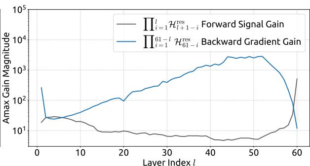
Source: Figure 3(b) of the paper. The composite mapping’s Amax gain (y-axis) across sub-layers of the 27B model. ① The unconstrained composite grows to ~3000× worst-case amplification. ② Layer index unrolls each Transformer block into Attention and FFN sub-layers.

The intuition: unconstrained residuals are like pipes whose diameter changes unpredictably at every joint — after 30 joints the flow rate is anyone’s guess.

A concrete example: the 12k-step loss surge and gradient-norm spikes in Figure 2 of the paper are the observable symptom of this composite gain. The gradient norm graph shows HC (orange) spiking far above the stable mHC/baseline profiles.

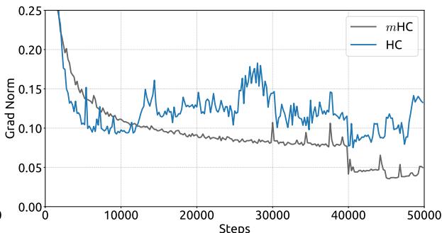
Source: Figure 2(b) of the paper. Gradient norm vs. training steps on the 27B model — unconstrained HC’s gradient norm explodes while mHC stays flat and baseline-like.

Remember: HC’s instability is a property of the composite, not of any single layer — that is why constraining each layer’s mixer is the right fix.

The doubly stochastic manifold: mHC’s core

What it does: mHC constrains \(\mathcal{H}_l^{\text{res}}\) to the set of doubly stochastic matrices: non-negative entries with every row and column summing to 1, i.e. the Birkhoff polytope \(\mathcal{P}_{\mathcal{M}^{\text{res}}}\).

Why it matters: this single constraint restores the identity-mapping property while keeping cross-stream mixing.

How it works: three formal properties do the heavy lifting:

Property	Statement	Consequence
Norm preservation	$|\mathcal{H}^{\text{res}}|_2 \le 1$	The mapping is non-expansive — no gradient explosion.
Compositional closure	product of doubly stochastic matrices is doubly stochastic	$\prod \mathcal{H}^{\text{res}}$ stays bounded over all depths.
Geometry	Birkhoff polytope = convex hull of permutation matrices	Mixing is a convex combination of streams; repeated application monotonically mixes information.

When $n=1$, the constraint degenerates to the scalar 1 — mHC exactly recovers the plain identity mapping. And because each $\mathcal{H}^{\text{res}}\mathbf{x}_l$ is a convex combination of the streams, the feature mean is conserved and the signal norm is strictly regularized.

The intuition: a doubly stochastic matrix is a “weighted shuffle” — it can redistribute energy between streams but can never create or destroy it.

A concrete example: in the 27B MoE, the composite gain for mHC peaks at ~1.6 instead of ~3000 — three orders of magnitude tighter, and the gradient norm stays flat and baseline-like.

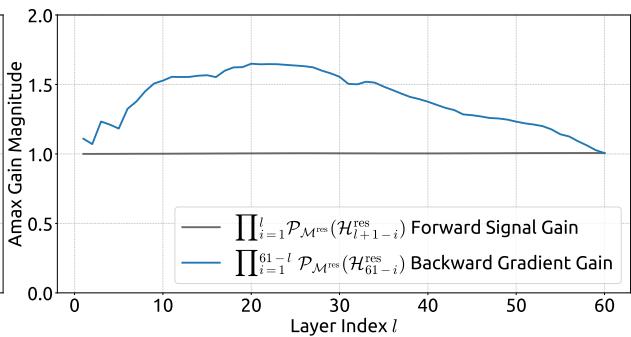
Source: Figure 7(b) of the paper. Same metric and model as Figure 3(b), but for mHC. ① The composite gain is bounded near ~1.6 (vs ~3000 for HC). ② The small residual deviation from 1.0 comes from the finite Sinkhorn-Knopp iterations.

Remember: doubly stochastic = non-expansive + composition-closed = the identity-mapping property, restored for free.

Sinkhorn-Knopp projection and parameterization

What it does: turns the raw learned mixer into a doubly stochastic matrix every forward pass.

Why it matters: the projection is what enforces the manifold; its efficiency decides whether mHC is practical.

How it works: mHC first flattens the stream state, computes dynamic + static parts (Eq. 7), then projects:

\[\mathcal{H}_l^{\text{res}} = \text{Sinkhorn-Knopp}(\tilde{\mathcal{H}}_l^{\text{res}}), \qquad M^{(0)} = \exp(\tilde{\mathcal{H}}_l^{\text{res}}), \qquad M^{(t)} = \mathcal{T}_r(\mathcal{T}_c(M^{(t-1)}))\]

with $t_{\max} = 20$ row/column normalization iterations ($\mathcal{T}_r$ = normalize rows to sum 1, $\mathcal{T}_c$ = normalize columns). The forward is a single fused kernel; the backward pass recomputes intermediates on-chip and traverses the whole iteration.

The intuition: exponentiate (make everything positive), then ping-pong row/column normalization until the matrix is doubly stochastic.

A concrete example: in the 27B model, the 20-iteration approximation leaves the backward (column-sum) gain slightly above 1 — the reason Figure 7(b) shows ~1.6 rather than exactly 1.0.

Remember: finite iterations buy speed at the cost of a tiny, bounded deviation from perfect conservation.

Non-negative pre/post mappings

What it does: mHC also constrains $\mathcal{H}^{\text{pre}}$ and $\mathcal{H}^{\text{post}}$ to be non-negative (sigmoid, and $2\sigma$ for post).

Why it matters: unconstrained pre/post coefficients can be negative and cancel signal when composed with the residual mixer.

How it works: the pre/post mappings use $\mathcal{H}^{\text{pre}} = \sigma(\tilde{\mathcal{H}}^{\text{pre}})$ and $\mathcal{H}^{\text{post}} = 2\sigma(\tilde{\mathcal{H}}^{\text{post}})$, guaranteeing all coefficients are positive.

The intuition: no negative weights means no destructive interference — every stream contributes constructively.

A concrete example: without this constraint, a negative write-back coefficient on one stream could subtract exactly what another stream added, silently wasting the stream’s capacity.

Remember: non-negativity on the gates is a second, cheaper manifold projection that removes signal cancellation.

Kernel fusion: making the wide stream cheap

What it does: mHC reorders and fuses the mapping computations so the $n \times C$ stream doesn’t multiply memory traffic.

Why it matters: the widened stream raises per-token I/O by roughly $n\times$ (Table 2 of the paper: HC’s total I/O goes from $2C$ read / $C$ write for residuals to $(5n+1)C$ read / $(3n+1)C$ write) — enough to kill training throughput without fused kernels.

How it works: three groups of fused kernels (implemented mostly in TileLang): ① fused scans computing $\tilde{\mathcal{H}}^{\text{pre}}, \tilde{\mathcal{H}}^{\text{post}}, \tilde{\mathcal{H}}^{\text{res}}$ plus the RMSNorm-scale in one pass over $\vec{\mathbf{x}}_l$, ② a single lightweight kernel for the small coefficient operations, ③ one kernel for the Sinkhorn-Knopp iteration with a custom recomputing backward. Fusing post/res with residual merging cuts the merge kernel’s reads from $(3n+1)C$ to $(n+1)C$ and writes from $3nC$ to $nC$. RMSNorm is reordered to divide by the norm after the matmul, preserving math while cutting latency on the $nC$-wide state.

The intuition: read the wide stream from memory once, do everything with it on-chip, write it back once.

A concrete example: on the 27B model the fused pipeline (load → cast → compute → store, mixed-precision: bf16 activations, tf32 projections, fp32 coefficients) is what brings total mHC overhead down to the headline 6.7%.

Remember: the 6.7% figure is not free — it is bought with kernel fusion, mixed precision, and careful scheduling.

Recomputing: trading memory for the transient

What it does: mHC discards the mHC kernels’ intermediate activations after the forward pass and recomputes them in the backward pass without re-running the heavy layer function $\mathcal{F}$.

Why it matters: the $n$-stream design multiplies activation memory; storing everything would force aggressive checkpointing.

How it works: for a block of $L_r$ consecutive layers, only the block input $\mathbf{x}_{l_0}$ is stored (every $L_r$ layers), plus each layer’s $\mathcal{F}$ output (per layer). The transient recompute memory is $(n+2)C \times L_r$, giving the optimal block size

\[L_r^{\star} = \arg\min_{L_r}\left[nC \left\lceil \tfrac{L}{L_r}\right\rceil + (n+2)C\,L_r\right] \approx \sqrt{\frac{nL}{n+2}},\]

which conveniently aligns with the layers-per-pipeline-stage.

The intuition: recompute the cheap mixer, keep the expensive layer output — memory drops without redoing $\mathcal{F}$.

A concrete example: with $n=4$ and the 27B’s 30 layers, recompute blocks line up with pipeline stages so the backward pass re-derives only the small mapping coefficients.

Remember: mHC recomputation is selective — it never re-runs attention or FFN, only the lightweight mixers.

Overlapping communication in DualPipe

What it does: mHC extends the DualPipe schedule so the extra cross-stage communication and stage-boundary recomputation overlap with compute instead of delaying it.

Why it matters: pipeline parallelism already moves activations between stages; an $n$-fold wider stream means $n$-fold more communication, and stage-boundary recomputation adds compute — both would enlarge pipeline bubbles.

How it works: ① the \(\mathcal{F}_{\text{post,res}}\) kernels of FFN layers run on a dedicated high-priority compute stream so the communication stream is never blocked; ② attention layers avoid persistent kernels so long-running attention can be preempted and flexibly scheduled; ③ recomputation is decoupled from pipeline communication because each stage’s initial activation \(\mathbf{x}_{l_0}\) is already cached locally.

Source: Figure 4 of the paper. F / B / W = forward, backward, weight-gradient computation. ① Attention (A) and MLP (M) kernel blocks are scheduled so communication overlaps with compute. ② mHC stage-boundary recomputation is decoupled from the communication stream.

The intuition: keep the network busy while the wide stream crosses stage boundaries — hide the cost instead of paying it serially.

A concrete example: without this, the 27B run’s stage-boundary recompute would serialize with gradient communication; with the extended DualPipe the two overlap and throughput stays at the 6.7%-overhead level.

Remember: mHC’s “only 6.7% overhead” claim depends on all three infrastructure pillars — fusion, recomputation, and DualPipe overlap — not just the math.

Putting It Together

Here is one forward + backward training step of the 27B MoE with mHC:

1. Stream in, mix: the $4 \times C$ stream state $\mathbf{x}_l$ enters the layer. The fused scan kernel computes $\tilde{\mathcal{H}}^{\text{pre}}, \tilde{\mathcal{H}}^{\text{post}}, \tilde{\mathcal{H}}^{\text{res}}$ in one pass (bf16 reads, tf32 projections, fp32 coefficients).
2. Project: the Sinkhorn-Knopp kernel runs 20 row/column normalizations, outputting the doubly stochastic $\mathcal{H}^{\text{res}}$.
3. Read out and compute: $\mathcal{H}^{\text{pre}}\mathbf{x}_l$ becomes the $1\times C$ layer input; attention or FFN runs on it and produces its output — the only activations stored per layer.
4. Merge back: the fused $\mathcal{F}_{\text{post,res}}$ kernel computes $\mathcal{H}^{\text{res}}\mathbf{x}_l + \mathcal{H}^{\text{post}^\top}\mathcal{F}(\cdot)$ in one read/write of the stream, keeping the convex-combination guarantee.
5. Forward all layers: each layer repeats 1–4; every block input $\mathbf{x}_{l_0}$ is kept per recompute block, nothing else from the mixers is stored.
6. Backward: the custom Sinkhorn-Knopp backward recomputes the projection on-chip; the two backward matmuls run as one fused kernel; mHC kernels re-execute without re-running $\mathcal{F}$.
7. Cross stage: at pipeline boundaries, FFN post/res kernels run on the high-priority stream while gradient communication overlaps; stage-local recomputation never waits on the network.
8. Result: stable gradient norms, no 12k-step loss surge, final loss 0.021 below the residual baseline — all at ~6.7% extra wall-clock time.

What This Buys You

The headline claim

mHC matches or beats unconstrained HC on downstream benchmarks while being stable enough to train at 27B scale — final training loss 0.021 lower than the residual baseline, and composite signal gain bounded at ~1.6 instead of ~3000.

How we know: 27B downstream benchmarks (Table 4)

Benchmark	27B Baseline	27B w/ HC	27B w/ mHC
BBH (EM, 3-shot)	43.8	48.9	51.0
DROP (F1, 3-shot)	47.0	51.6	53.9
GSM8K (EM, 8-shot)	46.7	53.2	53.8
HellaSwag (Acc., 10-shot)	73.7	74.3	74.7
MATH (EM, 4-shot)	22.0	26.4	26.0
MMLU (Acc., 5-shot)	59.0	63.0	63.4
PIQA (Acc., 0-shot)	78.5	79.9	80.5
TriviaQA (EM, 5-shot)	54.3	56.3	57.6

The mechanism behind the numbers

mHC outperforms HC on 6 of 8 benchmarks (notably +2.1 BBH, +2.3 DROP) and beats the baseline on all 8. The reasoning-heavy gains (BBH, DROP) are where deeper, stable stacks pay off: with bounded gradient flow the optimizer can train the full depth productively instead of compensating for exploding paths. The compute-scaling curve (3B → 9B → 27B) and token-scaling curve (3B on 1T tokens) both show the advantage persisting as compute grows — the property that made it worth deploying in DeepSeek-V4.

⚠️ How to read these numbers

• The 0.021 loss gap is vs. the residual baseline, not vs. HC. mHC’s stability advantage over HC shows up in training behavior (no loss surge, flat gradient norm), while the benchmark gap over HC is modest (+2.1/+2.3 on two tasks, −0.4 on MATH). Do not read “mHC beats HC everywhere” from the table.
• 6.7% overhead is for $n=4$ and includes the infrastructure work. Larger expansion rates or missing kernel fusion would change the number substantially.
• The ~3000 vs ~1.6 gain comparison is a worst-case metric, not average signal growth — but worst case is exactly what kills training.
• All models use DeepSeek-V3-style MoE with MLA; results may not transfer to dense architectures or other attention variants.

Where It Breaks

Failure mode	When it happens	Impact
Approximate Sinkhorn-Knopp	Only 20 iterations (the practical setting)	Backward gain drifts from 1.0, composite up to ~1.6 — still stable, but not exactly conservative
Recomputation blocks cross pipeline stages	Layer counts that don’t align with the optimal $L_r^{\star}$	Suboptimal memory/throughput tradeoff; stage-boundary recompute becomes a bubble
Expansion rate grows beyond 4	Wider streams need more I/O, more recompute, more communication	The 6.7% overhead does not hold; scaling may degrade
Unfused kernels	Any deployment skipping the TileLang fusion work	~$n\times$ memory-access overhead dominates; throughput collapses
Small models / $n=1$	Degenerate case	Recovers plain residual — no benefit, only added complexity
Non-MoE or non-pretraining regimes	Dense models, fine-tuning, or RL not covered by the paper	Stability claims validated for large-scale MoE pretraining only
In-house DeepSeek-V4 deployment	Production claims rely on the same infrastructure stack	The paper reports 6.7% on its own cluster; other clusters may differ

One Thing to Remember

mHC is the same hyper-connection topology as HC, but with the residual mixing matrix locked to the doubly stochastic manifold — a convex combination of streams that can never create or destroy signal, so composite gain stays near ~1.6 instead of exploding to ~3000. That single constraint restores the identity-mapping property that makes deep residual networks trainable, and with fused kernels, selective recomputation, and DualPipe overlap it costs only 6.7% wall-clock time — which is why DeepSeek shipped it in DeepSeek-V4.

Go Deeper

• Read: mHC: Manifold-Constrained Hyper-Connections (arXiv 2512.24880)
• Build on: Hyper-Connections (Zhu et al., 2024) — the unconstrained parent method; DeepSeek-V4 — the production deployment of mHC at 1.6T/284B scale
• Understand the context: Hyper-Connections (term) · DeepSeek-V3 (DualPipe) — the pipeline schedule mHC extends
• Reproduce: not available at time of writing