DeepSeek-V4: Million-Token Context via Hybrid Compressed Attention

Paper: DeepSeek-V4: Towards Highly Efficient Million-Token Context Intelligence Authors: DeepSeek-AI arXiv: Technical report, July 2026

TL;DR

What: DeepSeek-V4 is a family of Mixture-of-Experts LLMs — Pro (1.6T/49B activated) and Flash (284B/13B activated) — that natively support million-token contexts through a novel hybrid attention architecture.

How: Compressed Sparse Attention (CSA) uses chunked KV-cache compression to reduce the KV cache by 4× and applies sparse top-k selection; Heavily Compressed Attention (HCA) compresses by 128× with dense attention. Interleaving them across layers, plus Muon optimizer and manifold-constrained hyper-connections, yields dramatic efficiency gains.

The number: At 1M-token context, DeepSeek-V4-Pro uses only 27% of DeepSeek-V3.2’s single-token inference FLOPs and 10% of its KV cache size. DeepSeek-V4-Flash uses 10% FLOPs and 7% KV cache.

The Big Picture

DeepSeek-V4 Architecture

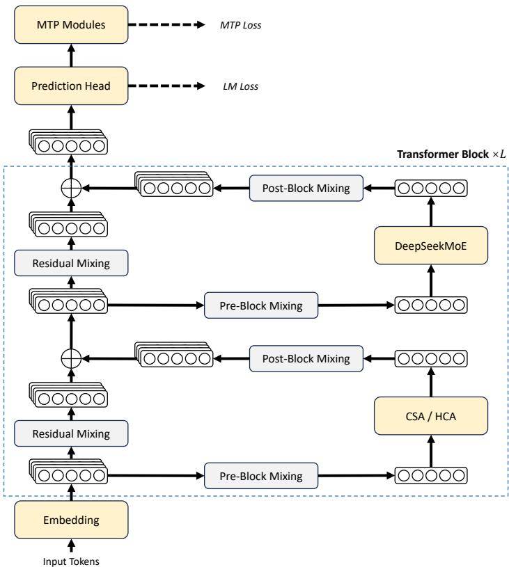
① DeepSeekMoE layers with shared + routed experts, Hash routing for early layers. ② Hybrid attention: interleaved CSA and HCA layers. ③ mHC replaces standard residual connections between blocks. ④ Muon optimizer (with hybrid Newton-Schulz iterations) replaces AdamW for most parameters. ⑤ Multi-Token Prediction (MTP) retained from V3.

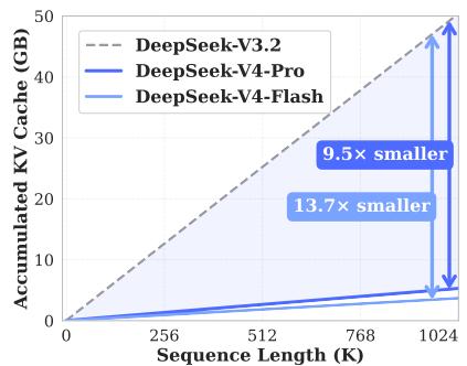
Benchmark and Efficiency Comparison

Left: benchmark performance of DeepSeek-V4-Pro-Max vs. counterparts. Right: inference FLOPs and KV cache size vs. DeepSeek-V3.2 — V4-Pro achieves 27% FLOPs and 10% KV cache at 1M tokens.

Why This Exists

Consider a standard LLM processing a 1-million-token context. With BF16 GQA8 (head dim 128) — a common configuration — each new token’s attention query must attend to 1M KV entries per layer, costing ~256 GB of KV cache and enormous FLOPs. Even DeepSeek-V3.2’s sparse attention struggles: at 1M context, it still needs substantial compute and cache. This makes practical deployment of ultra-long-context models economically infeasible.

Three problems compound:

Quadratic attention FLOPs dominate at long contexts, making token generation painfully slow.
KV cache memory grows linearly with sequence length, exhausting GPU HBM.
Training stability degrades with deeper, wider models, causing loss spikes that simple rollbacks can’t permanently fix.

DeepSeek-V4 tackles all three jointly: compressed attention crushes FLOPs and KV cache, mHC stabilizes deep signal propagation, and Muon accelerates convergence.

The Landscape

flowchart TD
    A[Vanilla Transformer Attention] --> B[MQA / GQA: share KV heads]
    A --> C[FlashAttention: IO-aware kernel]
    C --> D[FlashAttention-2/3/4: better parallelism, asynchrony]
    B --> E[MLA: low-rank KV joint compression]
    E --> F[DeepSeek-V2/V3: MLA + DeepSeekMoE]
    F --> G[DeepSeek-V3.2: DSA sparse attention]
    G --> H["DeepSeek-V4: CSA + HCA hybrid<br/>(compression × sparsity)"]
    B --> I[MiniMax Sparse Attention: block-sparse + index branch]
    I --> H
    C --> J["FP4/FP8 mixed precision attention"]
    J --> H

DeepSeek-V4 sits at the convergence of three evolutionary lines: (1) KV compression (MQA → MLA), (2) sparse attention (DSA, MSA), and (3) low-precision attention (FP8/FP4). Its key novelty is combining compression and sparsity in a hybrid, interleaved architecture — CSA layers compress lightly and select sparsely, while HCA layers compress aggressively and attend densely.

The Core Idea

Instead of choosing between dense attention (accurate but expensive), sparse attention (cheaper but risks missing important tokens), or KV compression (lossy but compact), DeepSeek-V4 interleaves them: CSA layers compress KV cache by 4× then select top-k blocks via a learned indexer, preserving fine-grained relevance; HCA layers compress by 128× and attend to everything, providing global context. Together with sliding-window branches for local dependencies, this gives the model both a “microscope” (recent tokens) and a “telescope” (compressed distant context) — all while keeping FLOPs and KV cache at fractions of V3.2 levels.

Symbol Map

CSA uses two KV series ($C^a$, $C^b$) with overlapping windows for compression; HCA uses a single series. Compression rates are $m$ for CSA and $m’$ for HCA.

Symbol	Human name	Shape / scope	Plain meaning
$m$	CSA compression rate	per-CSA-layer	Number of tokens compressed into one KV entry (4 in V4)
$m’$	HCA compression rate	per-HCA-layer	Number of tokens compressed into one KV entry (128 in V4)
$C^a, C^b$	KV entry series (a, b)	$n \times c$	Two KV series for CSA; $C^b$ overlaps with adjacent blocks
$Z^a, Z^b$	compression weights	$n \times c$	Learned weights determining how each token contributes to compressed entries
$C^{\text{Comp}}$	compressed KV entries	$\frac{n}{m} \times c$	Output of CSA/HCA compression, fed to core attention
$K^{\text{IComp}}$	compressed indexer keys	$\frac{n}{m} \times c^I$	Lower-dimensional keys used for sparse block selection
$c_t^Q$	latent query vector	per token, $d_c$	Shared compressed query representation for both indexer and core attention
$n_h$	query heads	per layer	Number of MQA query heads (64 Flash, 128 Pro)
$n_h^I$	indexer heads	per layer	Number of indexer query heads for sparse selection (64)
$n_{\text{win}}$	sliding window size	per layer	Number of uncompressed recent KV entries (128)

Deep Dive

Compressed Sparse Attention (CSA)

What it does: CSA compresses every $m$ tokens into one KV entry, then applies DeepSeek Sparse Attention (DSA) to select only the top-k compressed entries for core attention.

Why it matters: Naive compression loses fine-grained relevance between a query and specific tokens. CSA adds a learned Lightning Indexer that scores each compressed block against the query, selecting only the most relevant blocks — preserving accuracy while reducing the effective KV length by 4×, then further by the top-k ratio.

How it works:

Dual-series KV compression: Two independent KV series $C^a$ and $C^b$ are produced from input hidden states. Each compressed entry $C_i^{\text{Comp}}$ is a weighted sum of 2$m$ entries — $m$ from $C^a$ at positions $[mi, m(i+1)-1]$ and $m$ from $C^b$ at positions $[m(i-1), mi-1]$. The overlapping $C^b$ indices mean each compressed block shares information with its neighbor, softening the compression boundary.
Lightning Indexer: A separate compressed indexer key $K^{\text{IComp}}$ is produced (smaller head dim $c^I$). For each query token, indexer queries $\underset{t}{\mathbf{q}}^I$ are generated from a shared latent vector $\underset{t}{\mathbf{c}}^Q$. Per-block index scores $\underset{t,s}{I}$ aggregate over indexer heads with learned head weights.
Top-k selection: Only the top-k scoring compressed blocks participate in core attention. This is the sparse attention step — similar to DSA but operating on compressed blocks.
Core attention with shared KV MQA: The selected compressed entries serve as both keys and values in a Multi-Query Attention. All query heads share the same KV entries (MQA), but each head has its own query vector.
Grouped output projection: The $n_h$ output heads are split into $g$ groups, each projected to a smaller intermediate dimension $d_g$, then concatenated and projected to the full hidden size. This avoids the quadratic cost of projecting $c \cdot n_h$ dimensions directly.

CSA Architecture

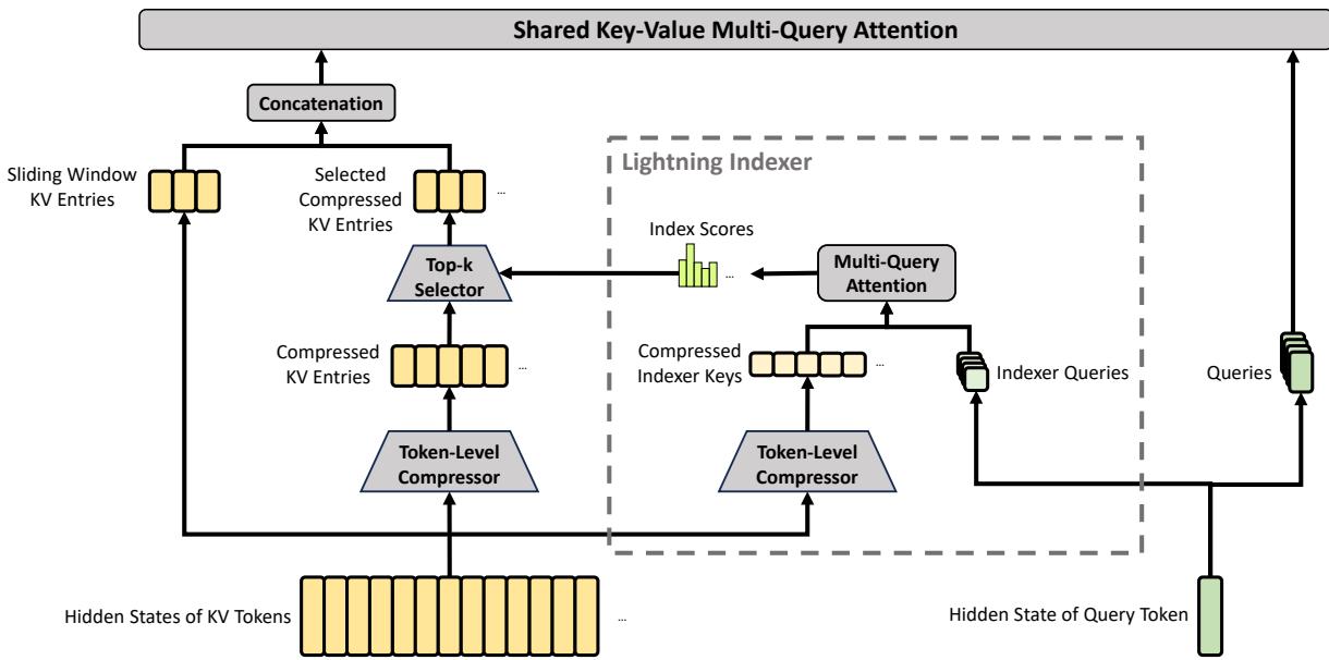
① Input hidden states generate two KV series and compression weights. ② Every $m$ tokens compress into one entry via softmax-weighted sum, with overlapping $C^b$ windows. ③ Compressed indexer keys enable sparse block selection. ④ Selected blocks feed MQA-style core attention with sliding-window KV entries. ⑤ Grouped output projection reduces parameter count.

The intuition: Think of reading a 10,000-page book. CSA is like summarizing every 4 pages into one paragraph (compression), then using a table of contents (indexer) to decide which summaries matter for answering your current question (sparse selection).

A concrete example: Processing a 1M-token legal document. Without compression, the attention module must store 1M KV entries per CSA layer and compute 1M attention scores per query. With CSA ($m=4$, top-$k$=512 for Flash, 1024 for Pro), the KV cache shrinks to ~250K entries, and each query only attends to 512-1024 of them. The sliding window branch ensures the model still sees the most recent 128 tokens at full fidelity.

Remember: CSA is “compress then select” — compression creates the candidates, the indexer picks which ones matter.

Heavily Compressed Attention (HCA)

What it does: HCA compresses every $m’$ tokens ($m’=128$, far larger than CSA’s $m=4$) into a single KV entry, then applies dense attention over all compressed entries.

Why it matters: At extreme sequence lengths, even CSA’s 4× compression leaves too many entries. HCA provides a second tier of compression that captures global, coarse-grained context at negligible cost — each HCA layer has only $\frac{n}{128}$ KV entries.

How it works:

Single-series aggressive compression: Unlike CSA’s overlapping dual-series approach, HCA uses a single KV series $C$ and compresses every $m’$ consecutive tokens into one entry via softmax-weighted sum. No overlap — each block is independent.
No sparse selection: HCA performs dense attention over all compressed entries. Since there are only $\frac{n}{128}$ of them, the FLOPs are manageable even without sparsity.
Identical downstream mechanics: HCA uses the same MQA, low-rank query projection, and grouped output projection as CSA. It also includes the sliding window branch for local dependencies.

HCA Architecture

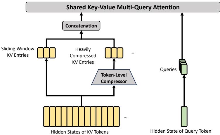
① Single KV series with compression weights. ② Every $m’$ tokens compress into one entry (no overlap). ③ Dense MQA-style attention over all compressed entries, plus sliding-window KV entries. ④ Grouped output projection.

The intuition: CSA is the “detailed summary” — you still have many entries but attend only to relevant ones. HCA is the “chapter outline” — you see everything at a very coarse grain.

A concrete example: In the same 1M-token legal document, an HCA layer produces only ~7,800 compressed entries. The model can attend to all of them densely, giving it global awareness of the entire document structure. Paired with CSA layers that zoom in on specific sections, this creates a two-scale attention system.

Remember: HCA trades per-token granularity for global coverage — it sees everything coarsely, while CSA sees selected things finely.

Hybrid Attention Configuration

What it does: CSA and HCA layers are interleaved across the Transformer stack, with the first two layers using special configurations.

Why it matters: Different layers capture different abstraction levels. Early layers benefit from local attention, mid layers mix global (HCA) and selective (CSA) views, and alternating them ensures the model has both fine-grained and coarse-grained context at every depth.

How it works (Flash / Pro):

Layers 1-2: Pure sliding window (Flash) or HCA (Pro)
Layers 3+: Interleaved CSA and HCA
Both models use $n_{\text{win}}=128$ for the sliding window branch

Remember: The hybrid interleaving is what makes the architecture work — CSA alone would miss global patterns, HCA alone would lose detail; together they form a multi-resolution attention pyramid.

Manifold-Constrained Hyper-Connections (mHC)

What it does: mHC expands the residual stream width to $n_{\text{hc}} \times d$ (where $n_{\text{hc}}=4$) and constrains the residual transformation matrix $B_l$ to the manifold of doubly stochastic matrices, preventing signal explosion or vanishing in deep stacks.

Why it matters: Standard residual connections can accumulate numerical instability across 43-61 layers. mHC’s doubly stochastic constraint ensures $\underset{2}{|\underset{l}{B}|} \leq 1$, making the residual transformation non-expansive — signals neither explode nor vanish during forward and backward passes. Both V4 models use $\underset{\text{hc}}{n}=4$.

How it works:

Expand: Residual state is widened from $\mathbb{R}^d$ to $\mathbb{R}^{n_{\text{hc}} \times d}$.
Dynamic parameterization: Input mapping $A_l$, residual mapping $B_l$, and output mapping $C_l$ are generated from both learnable static biases and input-dependent dynamic components.
Constrain: $B_l$ is projected onto the Birkhoff polytope (doubly stochastic matrices) via 20 Sinkhorn-Knopp iterations. $A_l$ and $C_l$ are constrained to $[0, 2]$ via Sigmoid.
Update: $X_{l+1} = B_l X_l + C_l \mathcal{F}_l(A_l X_l)$ where $\mathcal{F}_l$ is the layer operation (MoE or attention).

The intuition: Standard residuals are like a single pipe carrying signal between layers. If the pipe’s diameter can change unpredictably (unconstrained $B_l$), signal can explode or vanish. mHC uses 4 parallel pipes (the expanded stream) whose flow rates are constrained to sum to exactly 1 (doubly stochastic), guaranteeing stable propagation through arbitrarily deep stacks.

Remember: mHC is not about adding capacity — it’s about stabilizing signal flow through deep networks with minimal overhead (6.7% wall-time increase).

Muon Optimizer

What it does: Muon replaces AdamW for most parameters, using Newton-Schulz iterations to orthogonalize the momentum-accumulated gradient matrix before applying updates. This removes the need for per-parameter adaptive learning rates that AdamW maintains.

Why it matters: Muon converges faster and requires less tuning than AdamW. For trillion-parameter MoE models, faster convergence directly translates to fewer training tokens and lower cost.

How it works:

Accumulate momentum $M_t = \mu M_{t-1} + G_t$ (with Nesterov trick)
Orthogonalize: Apply 10 hybrid Newton-Schulz iterations — 8 steps with aggressive coefficients $(3.4445, -4.7750, 2.0315)$ for rapid convergence, then 2 steps with $(2, -1.5, 0.5)$ for precision
Rescale update RMS to match AdamW learning rate
Apply weight decay and update

The intuition: AdamW maintains per-parameter learning rates (memory-intensive for large models). Muon instead says: “just make the update matrix orthogonal, then scale it globally.” The Newton-Schulz iterations approximately compute $M(M^T M)^{-1/2}$, which is the optimal orthogonal approximation to $M$.

Remember: Muon uses hybrid Newton-Schulz (fast-then-precise), and DeepSeek-V4 can skip QK-Clip because its architecture already applies RMSNorm to attention queries and KV entries, preventing exploding logits.

Training Stability: Anticipatory Routing and SwiGLU Clamping

What it does: Two practical techniques prevent loss spikes in trillion-parameter MoE training.

Why it matters: Training V4 encountered instability where MoE routing amplified outliers, creating feedback loops that caused loss spikes. Simple rollbacks didn’t prevent recurrence.

Anticipatory Routing: At step $t$, use network parameters $\theta_t$ for features but routing indices from $\theta_{t-\Delta t}$. This decouples the feedback loop between backbone and routing updates. Activated dynamically — only when a spike is detected — with ~20% wall-time overhead during activation.

SwiGLU Clamping: Clamp the linear component of SwiGLU to $[-10, 10]$ and cap the gate component at 10. Empirically eliminates outliers without hurting performance.

Remember: Anticipatory Routing breaks the routing-feedback cycle; SwiGLU Clamping prevents individual activations from going pathological.

KV Cache Management

What it does: A heterogeneous KV cache design separates classical attention cache (CSA/HCA compressed entries) from state cache (SWA + uncompressed tail tokens), with on-disk storage for shared-prefix reuse.

Why it matters: Hybrid attention produces multiple KV entry types with different sizes, update rules, and eviction policies. PagedAttention can’t handle this diversity natively.

How it works: See the KV cache layout diagram.

KV Cache Layout

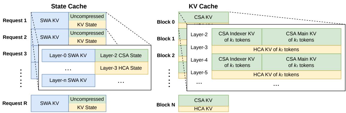
The KV cache is split: a state cache for SWA and uncompressed tail tokens (pre-allocated per sequence), and a classical KV cache for CSA/HCA compressed entries. Each classical cache block covers $\text{lcm}(m, m’)$ original tokens.

On-disk KV cache storage: For CSA/HCA, compressed entries are stored to disk and reused for shared prefixes. For SWA (8× larger volume), three strategies offer trade-offs: Full SWA Caching, Periodic Checkpointing, and Zero SWA Caching (recompute last $n_{\text{win}} \cdot L$ tokens using cached CSA/HCA entries).

Remember: The heterogeneous cache design is the engineering counterpart to the architectural innovation — without it, the hybrid attention’s efficiency gains can’t be realized in deployment.

Putting It Together

A query token at position 500,000 in a 1M-token context, in a CSA layer:

KV compression: The past 500K tokens have been compressed into ~125K CSA entries ($m=4$).
Lightning Indexer: The token’s latent query $\underset{t}{\mathbf{c}}^Q$ generates indexer queries — scores each compressed block, producing $\underset{t,s}{I}$.
Top-k selection: The top 1024 (Pro) or 512 (Flash) compressed blocks are selected.
Core attention: MQA over these 1024 compressed entries plus 128 sliding-window entries — total ~1152 KV entries to attend to (vs. 500K without compression/sparsity).
Output projection: Grouped projection reduces the $n_h \cdot c$ dimensional output efficiently.
Residual update: mHC mixes this attention output with the expanded residual stream via constrained $A_l, B_l, C_l$ mappings.

Result: Attention FLOPs are dominated by ~1152 entries instead of 500K. KV cache stores ~125K entries per CSA layer instead of 500K. And the model still has both global awareness (via HCA layers) and local fidelity (via sliding windows).

What This Buys You

The headline claim

DeepSeek-V4-Pro-Max redefines SOTA for open models, closing the gap with frontier proprietary models (Gemini 3.1-Pro, GPT-5.4) on reasoning while achieving dramatic efficiency gains at long contexts.

How we know: evidence summary

Category	V4-Pro-Max vs. Best Open	V4-Pro-Max vs. Best Closed
Knowledge (SimpleQA)	+20 pts over K2.6/GLM	Trails Gemini 3.1-Pro
Reasoning (Codeforces)	First open model matching GPT-5.4	On par (3206 vs 3168)
Reasoning (HLE)	Marginal lead over open	Trails Gemini 3.1-Pro
Agent (SWE-Verified, TerminalBench)	On par with K2.6, GLM-5.1	Trails Opus 4.5/4.6
Long-Context (MRCR 1M)	N/A (only V4 evaluated)	Beats Gemini-3.1-Pro (83.5 vs 76.3)
1M-token FLOPs	27% of V3.2 (Pro) / 10% (Flash)	—
1M-token KV cache	10% of V3.2 (Pro) / 7% (Flash)	—

The mechanism behind the numbers

The efficiency gains come from the hybrid attention’s combined effect: CSA gives 4× KV compression × top-k sparsity; HCA gives 128× KV compression. The interleaving means roughly half the layers get each benefit. Additional gains from FP8/FP4 mixed precision and the smaller attention top-k vs. V3.2.

The performance gains come from: Muon’s faster convergence on 32-33T tokens, mHC’s improved signal propagation enabling deeper/wider models, refined data quality, and the specialist-then-OPD post-training pipeline.

⚠️ How to read these numbers

The 27% FLOPs figure is measured in equivalent FP8 FLOPs. The FP4 × FP8 operations currently have the same peak throughput as FP8 × FP8 on existing hardware, but theoretically offer 1.33× more efficiency on future hardware. So the real-world speedup depends on hardware support for FP4 compute.

Where It Breaks

Failure mode	When it happens	Impact
Compression boundary artifacts	Tokens near block boundaries in CSA get $C^b$ from the previous block, not the current one	Boundary tokens may have less accurate KV representation
Top-k misses critical context	Indexer fails to select a compressed block containing needle-in-haystack information	Retrieval failure, especially beyond 128K context where performance degrades
Training instability without both mitigations	Only using Anticipatory Routing or SwiGLU Clamping alone	Loss spikes may recur; the paper found both techniques together are more robust than either alone
OPD mode collapse	Student learns to produce only high-probability tokens from one teacher, ignoring others	Loss of specialist diversity; the paper mitigates with full-vocabulary KL loss
SWA recomputation cost	Zero SWA Caching strategy requires recomputing $n_{\text{win}} \cdot L$ tokens per prefix hit	Higher prefilling latency for shared-prefix scenarios
Architecture complexity	The model uses CSA, HCA, mHC, Muon, hash routing, MTP — many interacting components	Harder to debug, ablate, and replicate; the paper acknowledges this and plans simplification
FP4 QK indexer recall	99.7% recall means 0.3% of KV entries are missed by the indexer	Minor accuracy loss in sparse selection, acceptable trade-off for 2× top-k speedup

One Thing to Remember

DeepSeek-V4 crushes the long-context efficiency barrier through interleaved compression and sparsity — CSA layers compress then select (detailed zoom), HCA layers compress then attend globally (wide panorama), and together with Muon, mHC, and FP4 precision they make million-token contexts not just possible but practical, at 10-27% the cost of the prior state of the art.

Go Deeper

DeepSeek-V4 open-source implementation
Model checkpoints on HuggingFace
DeepSeek-V3 Technical Report
DeepSeek-V3.2 (DSA) Technical Report
MiniMax Sparse Attention — A different sparse attention approach with an index branch and block-sparse KV selection
Muon Optimizer (Jordan et al., 2024)
mHC: Manifold-Constrained Hyper-Connections (Xie et al., 2026) — the mHC paper (arXiv 2512.24880) behind DeepSeek-V4’s residual mechanism
TileLang DSL (Wang et al., 2026)