GPipe: Micro-Batch Pipeline Parallelism

Paper: GPipe: Easy Scaling with Micro-Batch Pipeline Parallelism
Authors: Yanping Huang, Youlong Cheng, Ankur Bapna, Orhan Firat, Mia Xu Chen, Dehao Chen, HyoukJoong Lee, Jiquan Ngiam, Quoc V. Le, Yonghui Wu, Zhifeng Chen (Google)
arXiv: 1811.06965v5 (Jul 2019)

Related pages: Megatron-LM: GPU-Cluster Training Parallelism, Transformer

TL;DR

What: GPipe is a pipeline parallelism library that lets you train models larger than a single accelerator’s memory by splitting layers across devices and streaming microbatches through them — with synchronous gradient updates that guarantee correctness regardless of the number of partitions.

How: Partition the model into K sequential cells on K accelerators; split each mini-batch into M micro-batches; pipeline forward/backward passes so all accelerators stay busy; accumulate gradients across micro-batches and apply synchronously at the end of each mini-batch; use activation recomputation to slash memory.

The number: With $M \ge 4K$, the pipeline bubble overhead becomes negligible and throughput scales near-linearly — a 6.3× speedup on 8 TPUs for Transformer models, and 298× larger models (83.9B params) on 128 accelerators versus a single device.

The Big Picture

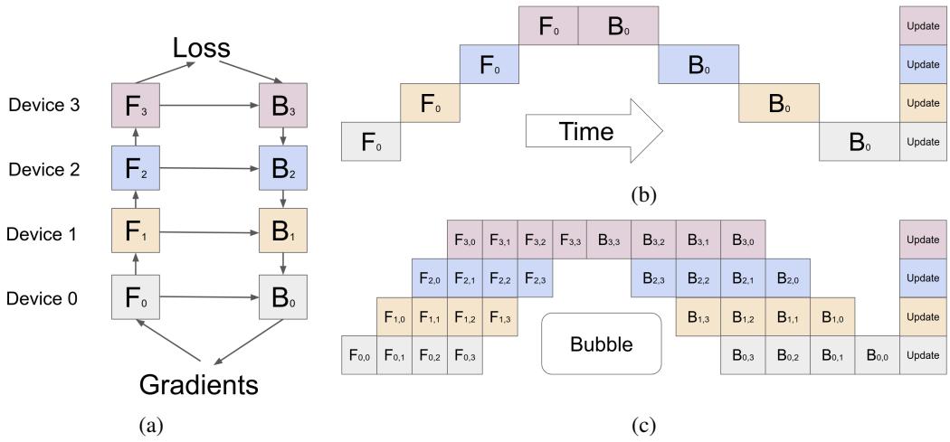
① A neural network is partitioned into K cells ($F_k$ = forward, $B_k$ = backward), each placed on a separate accelerator. ② Naive model parallelism leaves all but one accelerator idle at any moment. ③ GPipe splits the mini-batch into M micro-batches and pipelines them: as micro-batch 1’s forward pass finishes on device 1, device 2 starts its forward pass while device 1 begins micro-batch 2. During the backward pass, gradients flow in reverse. All gradients are accumulated and applied synchronously at mini-batch end.

Why This Exists

Imagine you want to train a 6-billion-parameter Transformer on 103 languages. A single GPU has 16 GB of memory. The model parameters alone consume ~72 GB (12 bytes each with optimizer state). You cannot even load the model, let alone compute activations.

Before GPipe, your options were:

• Data parallelism: Each GPU holds a full model copy. Requires the model to fit on a single device. Useless for giant models.
• Naive model parallelism: Split layers across GPUs. GPU 0 computes layer 0→1, sends activations to GPU 1, then sits idle while GPU 1 computes layer 2→3. At any moment, only one GPU works. 75% idle on 4 GPUs.
• Mesh-TensorFlow (SPMD): Split individual matrix multiplications across devices. Works but floods the interconnect with AllReduce traffic. Requires high-speed links. Architecture-specific.
• PipeDream: Pipelines forward and backward passes asynchronously. Higher utilization, but weight staleness means you need multiple parameter versions, eating memory and risking optimization issues.

GPipe solves this with synchronous pipeline parallelism: you get the utilization of pipelining without the correctness risks of async.

The Landscape

flowchart TD
  DP["Data Parallelism\n(each GPU holds full copy)"] --> SPMD["SPMD / Mesh-TensorFlow\n(split individual ops)"]
  DP --> MP["Naive Model Parallelism\n(split layers, sequential)"]
  MP --> PipeDream["PipeDream\n(async pipeline, weight staleness)"]
  MP --> GPipe["GPipe\n(sync pipeline, micro-batches, re-materialization)"]
  GPipe --> Megatron["Megatron-LM\n(TP + PP + DP, interleaved 1F1B)"]
  
  style GPipe fill:#d5e8d4,stroke:#82b366,stroke-width:2px

GPipe sits between naive model parallelism and Megatron-LM. It pioneered synchronous micro-batch pipeline parallelism. Megatron-LM later extended this with interleaved scheduling (1F1B) to further reduce the pipeline bubble.

The Core Idea

Instead of sending one giant batch through a pipeline and wasting GPUs at the head and tail, chop the batch into many small microbatches and stream them through like an assembly line. Make all gradient updates synchronous at mini-batch boundaries so the math is identical to single-device training. Add activation recomputation so you don’t need to cache intermediate activations — just recompute them during the backward pass.

The only cost is a “pipeline bubble” — the warmup and drain phases at the start and end of each mini-batch where not all accelerators are busy. Make the number of micro-batches M large enough (≥ 4K), and this bubble becomes negligible.

Symbol Map

Symbol	Human name	Meaning
$K$	number of partitions	How many accelerators the model is split across
$M$	number of micro-batches	How many pieces each mini-batch is divided into
$L$	number of layers	Total layers in the model
$N$	mini-batch size	Total training examples per gradient update
$F_k$	forward function of cell k	Composite forward computation for partition k
$B_k$	backward function of cell k	Gradient computation for partition k
$C_k$	cost estimator	Estimated FLOPs for partition k

Deep Dive

Partitioning and Cell Placement

What it does: Divides a sequence of L layers into K cells, placing one cell per accelerator.

Why it matters: The partitioning quality directly determines pipeline efficiency. Imbalanced cells create stragglers.

How it works: GPipe uses a cost estimator $c_i$ per layer to balance total estimated cost $C_k = \sum_{l=i}^{j} c_l$ across cells. Communication primitives are auto-inserted at partition boundaries — the user only specifies K, M, and the layer sequence.

The intuition: Think of it as load-balancing an assembly line. Each station should take roughly the same time.

Remember: Perfectly balanced cells give linear speedup; imbalanced cells (like AmoebaNet’s variable-width layers) give sub-linear scaling.

Micro-Batch Pipelining

What it does: Splits a mini-batch of size N into M equal micro-batches and pipelines them through K accelerators.

Why it matters: This is the mechanism that keeps all accelerators busy simultaneously, converting the naive sequential execution into a streaming pipeline.

How it works: During forward: accelerator k computes $F_k$ on micro-batch $m$, then sends output to accelerator $k+1$ and starts $F_k$ on micro-batch $m+1$. During backward: the process reverses, with $B_k$ depending on both the incoming gradient $B_{k+1}$ and the recomputed $F_k$. Gradients for all M micro-batches are accumulated and applied synchronously at mini-batch end.

The intuition: It’s an assembly line: each station works on a different unit simultaneously, and the final product (gradient update) only ships after all units pass through.

A concrete example: With K=4 accelerators and M=8 micro-batches, at steady state all 4 accelerators are computing simultaneously — accelerator 0 on micro-batch 8’s forward, accelerator 1 on micro-batch 7’s forward, accelerator 2 on micro-batch 5’s backward, accelerator 3 on micro-batch 3’s backward.

Remember: The pipeline bubble overhead is $O(\frac{K-1}{M+K-1})$. When $M \ge 4K$, it’s negligible.

Re-materialization (Activation Recomputation)

What it does: Each accelerator only stores output activations at partition boundaries; intermediate activations are recomputed during backward.

Why it matters: Without it, peak activation memory is $O(N \times L)$ — all activations for all layers. With it, memory drops to $O(N + \frac{L}{K} \times \frac{N}{M})$, enabling much larger models.

How it works: During forward, only the output of $F_k$ (the cell boundary activation) is saved. During backward, $F_k$ is recomputed from scratch to regenerate intermediate activations needed for $B_k$.

The intuition: Trade compute for memory. Activations are cheap to recompute but expensive to store.

A concrete example: On a single 8 GB GPU, the naive approach fits 82M parameters. With re-materialization alone, GPipe fits 318M parameters — a 3.9× improvement without adding devices.

Remember: Re-materialization works even on a single accelerator (K=1), cutting activation memory significantly.

Low Communication Overhead

What it does: Only transfers activation tensors at partition boundaries — no AllReduce, no parameter broadcasting.

Why it matters: Unlike SPMD approaches that need high-speed interconnects, GPipe achieves near-linear speedup even on PCI-E connected GPUs without NVLink.

How it works: Each cell boundary sends one activation tensor per micro-batch. That’s it. No gradient synchronization during the pipeline (gradients are local until mini-batch end).

The intuition: Pipeline parallelism trades more communication for more idle time when done poorly. GPipe minimizes both by only communicating at cell boundaries.

Remember: On 8 P100 GPUs without NVLink, GPipe still achieves 3.3× speedup for Transformer models — the communication bandwidth is not the bottleneck.

Putting It Together

A complete training step with GPipe:

1. Partition: Model is divided into K=4 cells. Each cell placed on one TPU.
2. Split: Mini-batch of N=128 examples split into M=32 micro-batches of 4 examples each.
3. Warmup (forward): Micro-batch 1 flows through cells 1→2→3→4. Micro-batch 2 follows, then 3, etc. After 3 steps (K-1), all 4 accelerators are busy simultaneously.
4. Steady state: All accelerators compute different micro-batches at different stages. Forward and backward overlap: cell 4 might be on micro-batch 3’s backward while cell 1 is on micro-batch 8’s forward.
5. Drain (backward): After the last micro-batch’s forward completes, backward passes cascade through cells 4→3→2→1.
6. Sync: Gradients from all 32 micro-batches accumulated. One synchronous parameter update applied across all accelerators. Identical to what single-device training would produce.

What This Buys You

Near-Linear Throughput Scaling

With M=32 micro-batches on 8 TPUs, Transformer training throughput scales 6.3× — close to the theoretical 8× maximum. AmoebaNet achieves 3.48× due to imbalanced layer costs.

K=	2	4	8
M=1 (no pipelining)	1×	1.07×	1.3×
M=4	1.7×	3.2×	4.8×
M=32	1.8×	3.4×	6.3×

Normalized Transformer training throughput on TPUs. When M ≫ K, the bubble shrinks and throughput approaches linear.

Massive Model Scaling

Configuration	Max Transformer Layers	Max Parameters
Single TPUv3 (16GB)	3	282M
GPipe, K=128	1663	83.9B

298× larger model on 128× more accelerators — near-perfect linear scaling for uniform architectures like Transformers.

Empirical Validation

• 557M AmoebaNet: 84.4% top-1 ImageNet accuracy (state-of-the-art at publication), with strong transfer to CIFAR-10 (99.0%), CIFAR-100 (91.3%), and 5 other datasets.
• 6B Multilingual Transformer: 128 layers, 102 languages → English. Outperforms bilingual baselines on 100 language pairs. Deeper models (24 layers, 8192 FFN dim) outperform wider models (12 layers, 16384 FFN dim) on low-resource languages, suggesting depth aids cross-lingual transfer.

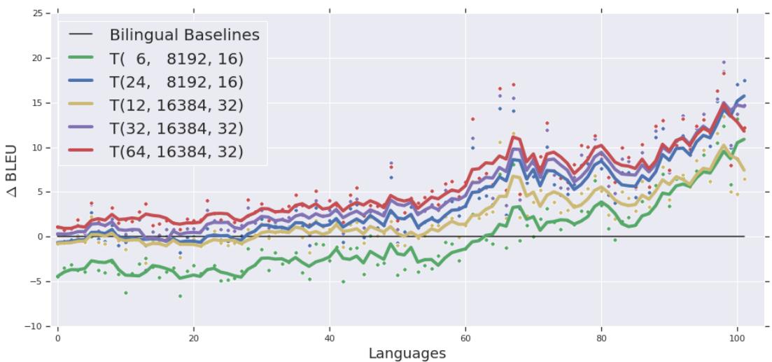
Translation quality (BLEU improvement over bilingual baseline) across 102 languages. Languages are arranged left-to-right by decreasing training data size. The 6B T(64, 16384, 32) model (red) consistently outperforms the 400M baseline (blue), with especially large gains for low-resource languages (right side).

• Large batch training: Scaling to 4M tokens per batch improves BLEU from 30.92 → 32.71 on German-English translation.
• Trainability fix for deep models: Logit clipping + layer-scaled initialization prevents the sharp-activation instability that kills deep Transformer training.

Design Trade-Offs vs. Alternatives

Approach	Gradient Correctness	Comm Overhead	Max Model Size	Architecture Flexibility
GPipe	✅ Synchronous	Low (boundary only)	~85B (128 TPUv3)	✅ Any sequential net
PipeDream	❌ Async (staleness)	Low	Limited by parameter versions	✅ Flexible
Mesh-TensorFlow (SPMD)	✅	High (AllReduce)	High (split individual ops)	❌ Architecture-specific
Data Parallelism	✅	High (gradient sync)	❌ Must fit on 1 device	✅ Flexible

Limitations

• Single layer must fit on one accelerator. If one layer’s memory exceeds device capacity, GPipe cannot help without further splitting.
• BatchNorm complications. Micro-batch statistics differ from mini-batch statistics. GPipe tracks per-micro-batch stats during training and accumulates mini-batch stats for evaluation.
• Partitioning quality matters. The cost estimation heuristic may produce imbalanced cells for irregular architectures like AmoebaNet, leading to sub-linear speedup.