Sequence Parallelism: Long Sequence Training from System Perspective

Paper: Sequence Parallelism: Long Sequence Training from System Perspective Authors: Shenggui Li, Fuzhao Xue, Chaitanya Baranwal, Yongbin Li, Yang You (National University of Singapore) arXiv: 2105.13120 (May 2021) Venue: ACL 2023

Related pages: Megatron-LM, GPipe, Transformer

TL;DR

What: Sequence parallelism splits the input sequence along the length dimension across GPUs so no single device holds the entire sequence — each GPU stores only its chunk and computes attention via ring-style P2P communication.

How: Ring Self-Attention (RSA) circulates key and value embeddings around a ring of GPUs in two passes: first for $QK^T$ scores, second for the weighted $AV$ output. Each GPU accumulates partial results without ever needing the full $L \times L$ attention matrix locally.

The number: On 64 P100 GPUs, sequence parallelism achieves 13.7× larger batch size and 3.0× longer sequence length than tensor parallelism; with sparse attention it handles 114K+ tokens — 27× longer than single-device approaches.

The Big Picture

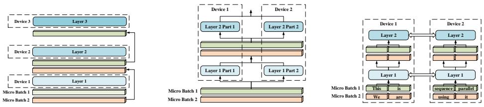
Pipeline parallelism (a) splits by layer, tensor parallelism (b) splits weight matrices by column/row, and sequence parallelism (c) splits the input sequence into chunks. All devices in (c) hold identical model parameters but different sub-sequences.

Sequence parallelism fills a gap in the parallelism taxonomy. Pipeline parallelism splits the model vertically (by layers); tensor parallelism splits model weights horizontally (by hidden/head dimensions); sequence parallelism splits the data along a new axis — sequence length. This makes it orthogonal to the other three paradigms, enabling true 4D parallelism: data + pipeline + tensor + sequence.

Why This Exists

Consider training a vision Transformer on a 3D medical scan of size $512 \times 512 \times 512$. Flattened into patches, this produces over 500× more tokens than a typical $256 \times 256 \times 3$ image. A single GPU at batch size 1 would need to store:

• The $L \times L$ attention matrix: $512^3 \times 512^3$ entries — completely infeasible
• Even for $L = 2048$, the attention matrix alone is ~32 MB per head in FP16. With 12 heads, that’s ~384 MB — and the MLP activations, optimizer states, and gradients push it past a 16 GB P100.

Existing parallelism (tensor, pipeline) was designed for model size, not sequence length. Tensor parallelism splits attention heads — but the number of heads (e.g., 12) is far smaller than the sequence length (e.g., 2048+). Pipeline parallelism splits layers — but each device still holds the full activation tensor for its stage. Neither helps when the sequence itself is too long for one GPU.

The Landscape

flowchart TD
  DP[Data Parallelism] --> SP
  PP[Pipeline Parallelism<br/>GPipe, 2018] --> SP
  TP[Tensor Parallelism<br/>Megatron-LM, 2019] --> SP
  SA[Sparse Attention<br/>Linformer, BigBird, 2020] --> SP

  SP[Sequence Parallelism<br/>Li et al., 2021] --> 4D[4D Parallelism<br/>DP + PP + TP + SP]

  DP -->|replicates model| 4D
  PP -->|splits by layer| 4D
  TP -->|splits by hidden/head dim| 4D
  SP -->|splits by sequence length| 4D

Sequence parallelism is not a replacement but a fourth dimension. Tensor parallelism splits along attention heads ($Z$) and hidden size ($H$), both small hyperparameters that cap scalability (max 12-16 GPUs for BERT). Sequence parallelism splits along sequence length ($L$), which is typically much larger. Pipeline parallelism splits along depth; sequence parallelism is orthogonal, and the two compose naturally — since activations are already chunked by sequence, there’s no need to split/all-gather them between pipeline stages (unlike tensor parallelism, which pays this extra cost).

Sparse attention (Linformer, BigBird) reduces the algorithmic complexity of attention from $O(L^2)$ to $O(L)$. When combined with sequence parallelism, the memory per device scales as $O(L/N)$ instead of $O(L)$, meaning you can in theory train with arbitrarily long sequences by adding more GPUs.

The Core Idea

Instead of storing the full $L \times L$ attention matrix on one GPU, split the sequence into $N$ chunks of length $L/N$ across $N$ GPUs. Each GPU holds its chunk’s $Q$, $K$, $V$. To compute the full attention output for chunk $n$, that GPU needs dot products between its $Q^n$ and everyone else’s $K$ and $V$. The insight: circulate $K$ and $V$ around a logical ring so each GPU sees them all, one neighbor at a time, without ever materializing the full matrix anywhere.

Row split, not column split. $Q^n, K^n, V^n$ each have shape $(B, Z, \frac{L}{N}, A)$ — the sequence length $L$ is divided into $N$ equal chunks, while the head dimension $A$ and the number of heads $Z$ remain whole on every device. This is a row-wise partition of the $(L, d)$ embedding matrix: each GPU owns $\frac{L}{N}$ rows (tokens) with all $d$ feature columns. Contrast with tensor parallelism, which column-splits weight matrices — dividing heads or hidden dimensions — and with pipeline parallelism, which splits by layer depth.

Symbol Map

Symbol	Human name	Shape / scope	Plain meaning
$N$	number of GPUs	scalar	Number of devices in the sequence-parallel group.
$L$	sequence length	scalar	Total number of tokens in the input sequence.
$B$	batch size	scalar	Number of sequences processed together.
$H$	hidden size	scalar	Dimension of the Transformer’s hidden states.
$Z$	number of attention heads	scalar	How many parallel attention heads.
$A$	attention head size	scalar	Dimension per head ($H = Z \cdot A$).
$Q^n, K^n, V^n$	chunk embeddings	$(B, Z, L/N, A)$	Query/key/value for the $n$-th sequence chunk on device $n$.
$S^n$	partial attention scores	$(B, Z, L/N, L)$	Full-row attention scores for chunk $n$, assembled incrementally.
$S_i^n$	column-split scores	$(B, Z, L/N, L/N)$	One block of $S^n$ corresponding to chunk $i$’s keys.
$O^n$	chunk output	$(B, Z, L/N, A)$	Final attention output for chunk $n$.

Deep Dive

Ring Self-Attention (RSA)

RSA has two communication stages, each requiring $N-1$ ring hops:

Stage 1: Score computation (circulate $K$). Each device $n$ starts with its local $(Q^n, K^n)$. It computes the partial score $S_n^n = Q^n (K^n)^T$. Then it sends $K^n$ to device $(n+1) \bmod N$ and receives $K^{n-1}$ from device $(n-1) \bmod N$. It computes $S_{n-1}^n = Q^n (K^{n-1})^T$ and concatenates. This repeats $N-1$ times. At the end, each device has the full $S^n \in \mathbb{R}^{L/N \times L}$ for its chunk.

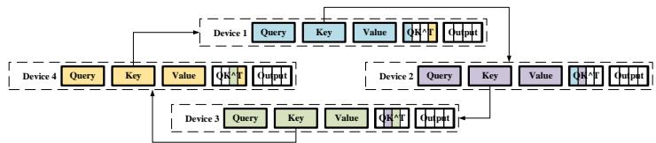
① Each device starts with its local $K$ and computes $QK^T$ locally. ② $K$ is sent to the next device around the ring. ③ Each device computes $QK^T$ with the received $K$. ④ After $N-1$ hops, each device has the full attention score matrix for its chunk.

Stage 2: Output computation (circulate $V$). Now each device has $S^n$ but needs to multiply it by all $V^1, \dots, V^N$. The same ring pattern circulates $V$ embeddings. Each device computes a partial $S_i^n V_i$ and accumulates:

\[O^n = \sum_{i=1}^{N} S_i^n V_i\]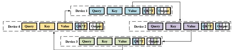

① Each device holds its full $S^n$ and its local $V$. ② $V$ circulates around the ring. ③ Each device computes the partial weighted sum $S_i^n V_i$ and accumulates. ④ After $N-1$ hops, each device has the final attention output $O^n$ for its chunk.

After RSA, each device has $O^n$ — the attention output for only its chunk. The MLP blocks that follow operate trivially on each chunk independently, with no communication needed (unlike tensor parallelism, which requires all-reduce in both MLP layers).

Memory Analysis: When Sequence Parallelism Wins

The memory advantage depends on the relationship between batch size, sequence length, and hidden dimensions:

• MLP block: Sequence parallelism wins when $BL > 32H$. For BERT Base ($H=768$), this means any $(B,L)$ pair where $B \cdot L > 24{,}576$ — almost always true.
• Attention block: Sequence parallelism wins when $BL > 16AZ$. For BERT Base ($A=64, Z=12$), this is $BL > 12{,}288$ — also almost always true.

The intuition: tensor parallelism splits weight matrices (saving parameter and optimizer memory), while sequence parallelism splits activations (saving the memory that scales with $B$ and $L$). For long sequences, activation memory dominates, making sequence parallelism the right choice.

Communication Cost

Surprisingly, sequence parallelism has the same total communication volume as tensor parallelism: both transfer $8(N-1) \cdot B \cdot Z \cdot (L/N) \cdot A$ bytes per Transformer layer (forward + backward). However:

• Tensor parallelism needs all-reduce in both MLP and attention blocks
• Sequence parallelism needs ring P2P only in attention — MLP has zero communication
• When combined with pipeline parallelism, tensor parallelism must split-then-all-gather activations between pipeline stages; sequence parallelism skips this because activations are already chunked

This gives sequence parallelism a throughput advantage when composed with pipeline parallelism (see Figure 4b in the paper).

Empirical Results

Maximum batch size (BERT Base, 64 GPUs): 13.7× larger than tensor parallelism. Tensor parallelism is capped at 12 GPUs (limited by attention heads); sequence parallelism scales to 64 GPUs because $L$ is much larger than $Z$.

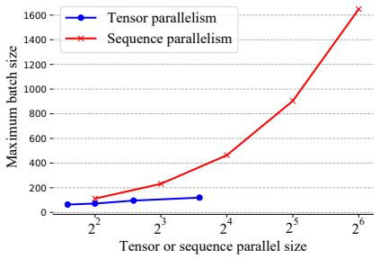
Sequence parallelism (orange) continues scaling past tensor parallelism’s head-count limit (12 GPUs), reaching 13.7× larger batch size at 64 GPUs.

Maximum sequence length (BERT Base, 64 GPUs): 3.0× longer than tensor parallelism. Even at the same GPU count (16 GPUs), sequence parallelism handles 1.4× longer sequences.

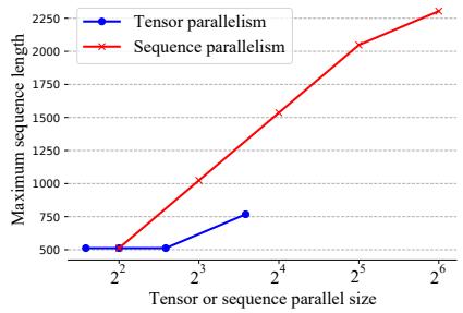
Sequence parallelism handles longer sequences than tensor parallelism across all GPU counts. The gap widens with more GPUs — sequence parallelism is not bottlenecked by small hyperparameters like attention head count.

With sparse attention (Linformer, 32 GPUs): Handles sequences of 114K tokens — 27× longer than single-device sparse attention approaches. The memory for sparse attention with sequence parallelism scales as $O(L/N)$, enabling theoretically infinite-length training.

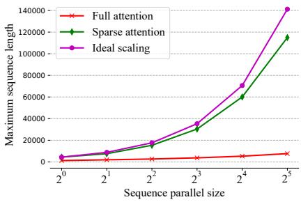
With sparse attention, sequence parallelism achieves near-ideal scaling — linear growth in maximum sequence length with GPU count, breaking past 100K tokens at 32 GPUs.

Weak Scaling

In weak scaling experiments (batch size proportional to GPU count), sequence parallelism maintains nearly constant memory per GPU as the global batch size grows — tensor parallelism memory grows and eventually OOMs. For sequence-length weak scaling (longer sequences on more GPUs), memory per GPU grows sub-linearly with sequence length.

Convergence

The authors verified that sequence parallelism produces equivalent training dynamics to tensor parallelism on BERT Large, with similar MLM and SOP loss curves over 50K iterations. This is expected — sequence parallelism is a system-level optimization that computes exactly the same forward pass as a single-GPU model (just distributed), so there should be no accuracy difference beyond floating-point non-determinism.

Integration with 4D Parallelism

Sequence parallelism composes with the three existing dimensions:

Dimension	What it splits	Bottleneck
Data parallelism	Batch	Communication bandwidth
Pipeline parallelism	Layers	Pipeline bubble
Tensor parallelism	Hidden/head dims	Small $Z, H$ cap scalability
Sequence parallelism	Sequence length	Ring communication overhead

Since sequence parallelism splits along $L$ (typically the largest dimension), it has the highest scalability ceiling. The paper envisions combining all four into 4D parallelism for training extremely large models on very long sequences — a vision later realized by systems like Megatron-LM (which adopted sequence parallelism in later versions).

Limitations

• Ring communication overhead: RSA requires $2(N-1)$ P2P messages per forward pass, which can become a bottleneck at very large $N$ or when inter-node bandwidth is limited.
• Only for bidirectional attention: The paper focuses on bidirectional (BERT-style) self-attention. Causal (GPT-style) attention requires adaptation — the ring pattern still works but can be optimized since each token only attends to previous tokens.
• Evaluated on BERT only: All experiments use encoder-only models. Scaling behavior on decoder-only or encoder-decoder architectures is not characterized.
• P100-era benchmarks: Experiments ran on 16 GB P100 GPUs. Modern GPUs (80 GB A100/H100) would shift the memory crossover points, potentially favoring tensor parallelism at moderate sequence lengths.
• No 4D integration results: The paper proposes 4D parallelism but only evaluates SP + PP and SP standalone. Full DP+PP+TP+SP integration is left as future work.

References

• Shoeybi et al., “Megatron-LM: Training Multi-Billion Parameter Language Models Using Model Parallelism,” arXiv:1909.08053, 2019. — Tensor parallelism baseline.
• Huang et al., “GPipe: Efficient Training of Giant Neural Networks Using Pipeline Parallelism,” NeurIPS 2019. — Pipeline parallelism framework.
• Wang et al., “Linformer: Self-Attention with Linear Complexity,” arXiv:2006.04768, 2020. — Sparse attention used in the 114K-token experiment.
• Zaheer et al., “Big Bird: Transformers for Longer Sequences,” NeurIPS 2020. — Alternative sparse attention baseline.
• Narayanan et al., “Efficient Large-Scale Language Model Training on GPU Clusters,” arXiv:2104.04473, 2021. — Megatron-LM v2 with PTD-P parallelism.